Part 2: Fundamental Aspects of MD Simulations

In the last part we understood the thermodynamic background and evolution of MD simulations technique. Here, we will look into some of the early challenges and developments in MD simulations. We will then understand some of the basic concepts and steps involved in performing a successful simulation.

Early Simulations:

Before the 1940s, generally, people carried out analytical calculations manually. In most cases, women performed the computation under the lead of physicists. Around the late 1940s, electronic digital machines called computers became common and revolutionized the way physicists approached solving many-body problems. Calculations finally became mechanized.

During WW2, mathematicians Jon Von Neumann and Stanislaw Ulam encountered the problem of studying neutron diffusion. The problem was too complex for analysis by trial-and-error method. So, they decided to go by the technique Roulette Wheel where the essential data about the occurrence of various events were known. The probabilities of separate events were merged in a step-by-step analysis to predict the outcome of the whole sequence of events. Upon applying the technique, they found tremendous success. This technique became popular and found application in various aspects of research studies.

Following the success of earlier simulations using the Monte Carlo method, Molecular Dynamics (MD) simulations began to be used around the 1950s. The first paper based on MD was published in 1957 by B.J. Alder and T.E. Wainwright where they studied phase transition of hard-sphere systemsⁱ. Later, Aneesur Rahman published Correlations in the motion of atoms in Liquid Argon in 1964. Stillinger published a paper in 1974 on Improved simulation of liquid water by molecular dynamics.

In the 1970s, biophysicists and biochemists started using MD. The first MD simulation on protein folding was carried out in 1975 and got published in Nature. Later, in 1976 simulation of a biological process was carried out. It showed that protein motion heavily influences biological processes. In 2013, Martin Karplus, Michael Levitt, and Arieh Warshell jointly received the Nobel Prize in Chemistry for their significant contribution to the development of multiscale models for complex chemical systemsⁱⁱ.

But what is Molecular Dynamics?

Martin Karplus once referred, “Molecular dynamics (MD) simulations predict how every atom in a protein or other molecular system will move over time based on a general model of the physics governing interatomic interactions.”ⁱⁱⁱ

Simply put, it is a computational technique where the motion of a particle or a collection of particles like atoms and molecules in a system is imitated under the influence of interatomic potentials to study various thermodynamic/structural and dynamic properties of a system of interest.

Why MD instead of Monte Carlo?

The best way to describe the difference between Monte Carlo and Molecular Dynamics simulation is by comparing a film trailer with that of the whole film itself.

In the trailer, we see random video footage such that we get the overall vibe of the storyline and judge whether the whole film is interesting enough to watch or not.

While watching the entire film, we witness how the characters developed over time; how they interacted with their surroundings and fellow beings under the given circumstances. At the end of the film, we know whether the character was a tragic hero or a villain, alive or dead.

The Monte Carlo technique employs a random sampling method where one configuration that is a snapshot of the simulated system of particles is not linked to the other over time. It is like looking at the movie trailer that randomly displays footage to pique our curiosity to watch the whole film. It provides information about thermodynamic properties only.

In molecular dynamics, like the entire movie itself, configurations are chronologically stored that provide us with data for both thermodynamic and transport properties like diffusivity, etc.

For example, if we want to know how a protein folds, we need to use MD. But if we only want to know whether a protein folds or not, simply Monte Carlo will be enough.

MD simulation basics

One can measure the force exerted on each particle in the system by the rest if their position coordinates are known. Then we can numerically forward integrate Newton’s second laws of motion to predict the spatial position of each particle as a function of time. In each step of the simulation, the computer calculates the intermolecular forces. After that, updates the resultant velocity and position for each particle. The resulting trajectory is a 3D movie that describes the atomic-level configuration of the system at every point during the simulated time interval.

One performs several statistical analyses to understand the thermodynamic and transport properties of the system using the resultant trajectory when the simulation finishes. Thermodynamic properties include observables like excess enthalpy, excess density, etc. Transport properties include diffusivity, hydrogen bond lifetime correlation, etc.

Now, the result from a simulation depends upon the choice of the molecular mechanics force field used. The molecular mechanics force field is a model that describes how forces are to be calculated during a simulation.

Force field is much like a recipe book that has the details like shape, size, weight, etc., of the required ingredients to prepare the dish. The details in a force field are based on quantum mechanical calculations or some other experiments.

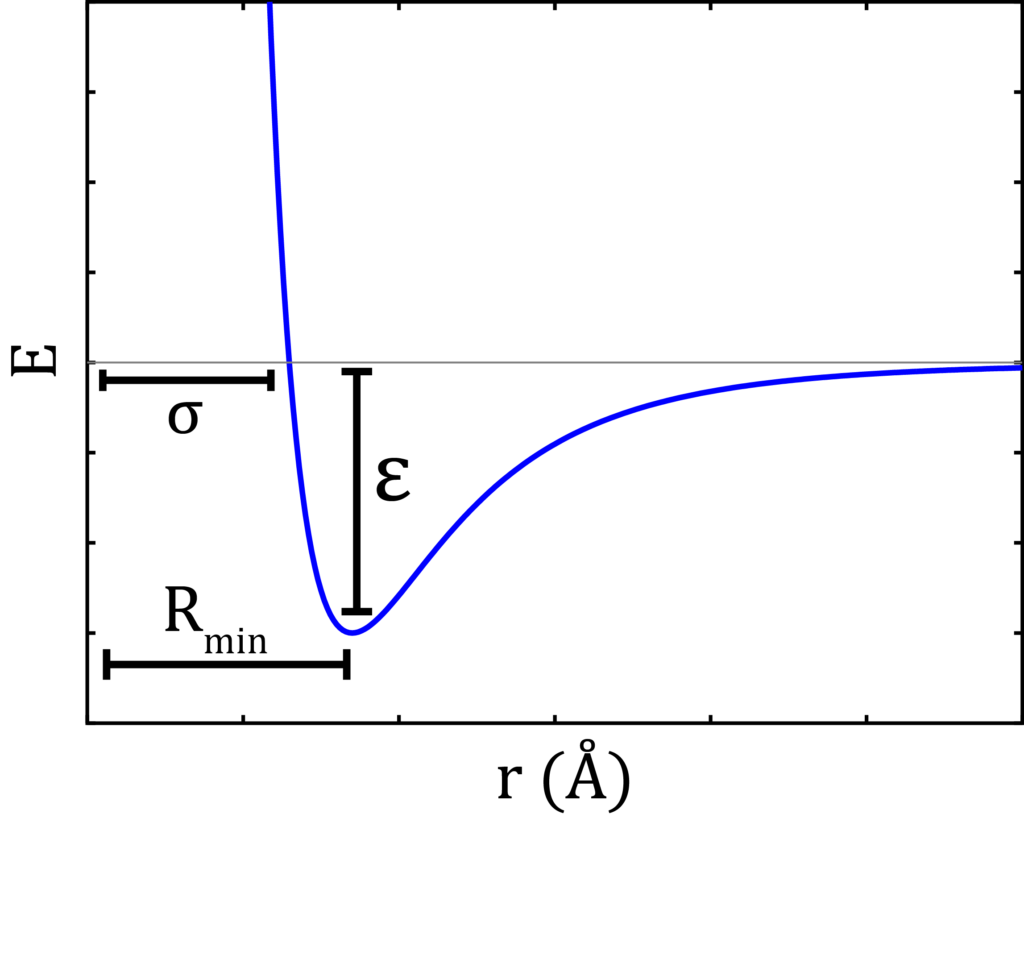
A typical force field contains the partial charge of each atom of molecules to be simulated. Bond angle and bond distance describe the shape and size of the molecules. A force field also quantitively depicts the values of potential well depth (ε) and collision diameter (σ).

One of the jobs of MD simulation is to measure the interaction potentials of the molecules present in the system. Interaction potentials are classified in two ways – intramolecular and intermolecular. The first one measures the interaction between the sites present in the same molecule. The bending potential and dihedral potentials are examples of it.

Intermolecular potentials measure the potential between the sites of different molecules. They include long-range electrostatic interactions through Coulomb potential and short-range potential like van der Waals interaction.

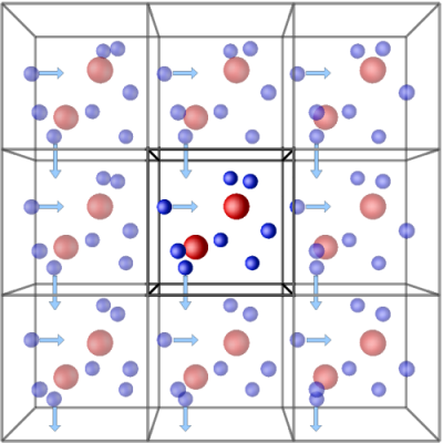
V(r) = 4ε[(σ/r)12-(σ/r)6]

Another feature of simulation is that one can study the properties of an ocean by merely looking into a glassful of water! Simulations should perform such that they are realistic. They should moderately reproduce the features of the real system and finish within a considerable time. A simulation of a single, large system will always be more computationally expensive than a smaller one as the larger system will have more particles hence more pairs for the calculation of interaction potentials. So, to reduce computation time, a large system can be smartly reduced to smaller repetitive units using a technique called periodic boundary condition (PBC)^iv.

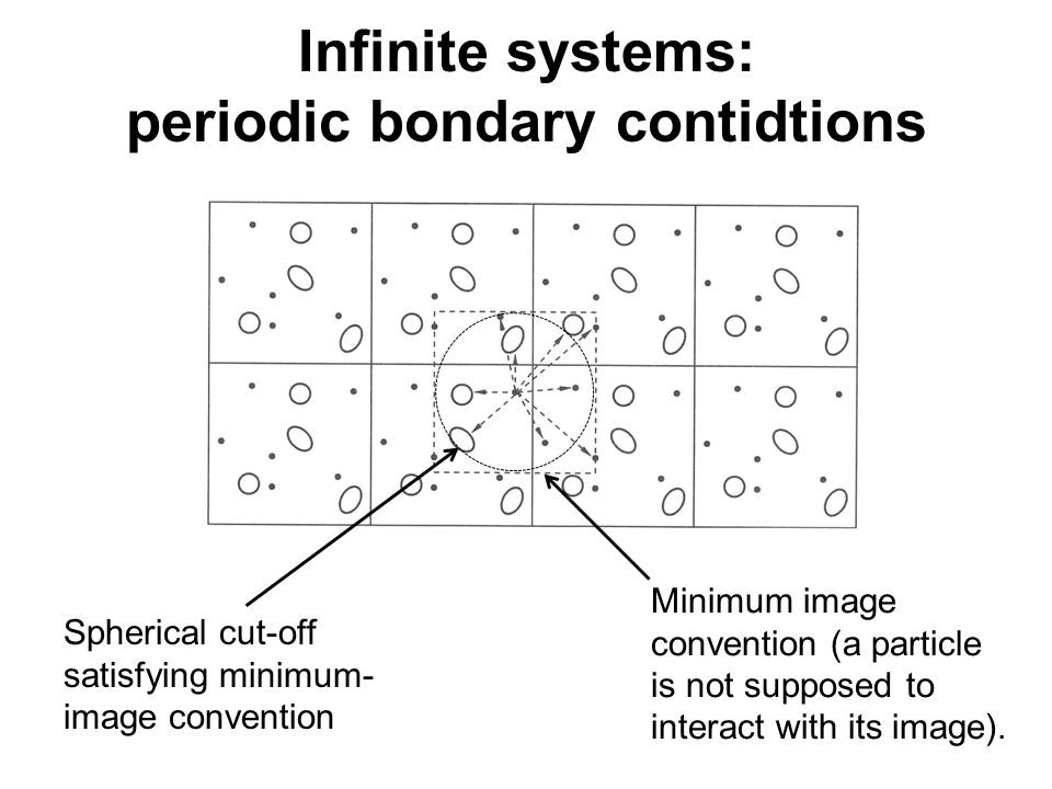
Generally, PBC is used to study the bulk properties of a system. It is a technique where a simulation box is translated infinitesimally in all directions in three-dimensional space. It is constructed such that the number of particles that leave the central box remains the same as that entering the adjacent box in the opposite direction. This way number of particles in the system is kept constant.

However, this technique has limitations. Simulations involving PBC pose difficulty in studying systems that approach phase transition. Because PBC is concerned with bulk properties and not interfacial phenomena. It also suppresses correlations that are larger in length than the size of the system. As a result, during phase transitions, the results upon studying large-scale correlated fluctuations become erroneous.

Another aspect of MD simulation is minimum image convention. PBC leads to an infinite number of interacting pairs. Thus, the calculation potential for all these pairs is very computationally expensive. To address the issue, depending upon the type of potential used, a cut-off region around each particle is assigned. Usually, the cut-off region is equal to or less than half of the simulation box length. Interaction potential is only calculated if the molecules lie on and within the boundary of the cut-off region. Rest is set to zero.

The minimum region may contain particles belonging to both real and periodic images. Also, one particle must not interact with its image. This way a lot of time is saved and hence the efficiency of performance is improved.

Where to set the boundary?

Generally, the particle in one corner of the simulation box does not interact with another lying at another corner of the box for short-range potentials. Such pairs do not contribute much to the total energy of the system. We can truncate the intermolecular interaction by applying a cut-off distance. However, for long-range interactions, special corrections like Ewald^v, particle mesh Ewald are applied.

The relationship between timestep interval and simulation result is like that of a fountain pen, paper, and the writing experience. To enjoy a good writing experience, the page quality is equally important as the pen itself. An expensive pen will be of no use if the ink bleeds through the paper. Likewise, no meaningful information can be extracted from the simulation if the timestep is not correctly set. Thus, the choice of timestep is crucial for an MD simulation.

The timestep (∆t) is the interval during the simulation at which the numerical integration of forces is carried out; followed by reassignment of the coordinates and the velocity of the particles in the system. Quoting the words of David Fincham^vi:

The use of finite difference algorithms to integrate the equations of motion in a series of timesteps inevitably leads to some error in the molecule trajectories which will depend both on the integrations algorithm used and on the choice of the timestep. …. The larger the value of ∆t which can be used rapid is the sampling of phase space, reducing the requirements for computer time.

David Fincham (Comp. Phy. Comm. 40, 1986, 263—269)^vi

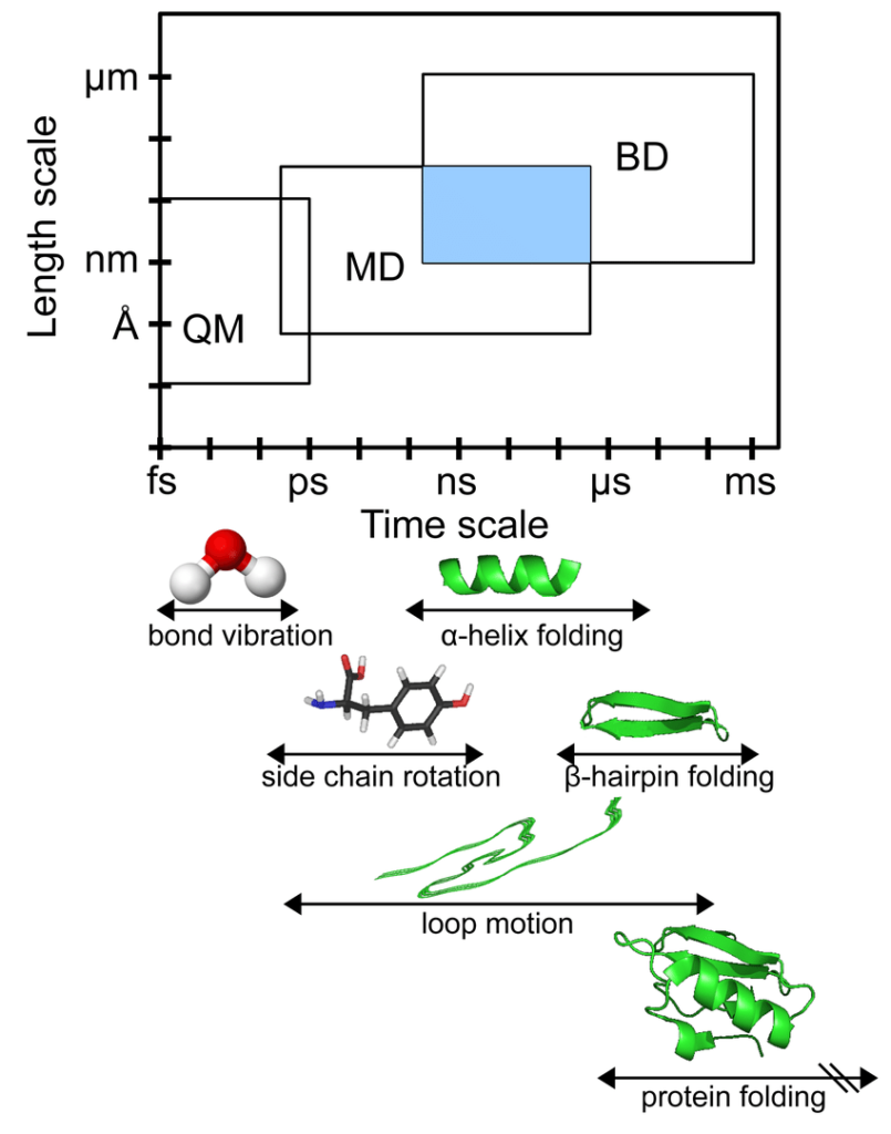
The time steps in an MD simulation must be short, typically only a few femtoseconds to ensure numerical stability. Most of the biochemical events like structural changes in proteins take place on timescales of nanoseconds, microseconds, or longer.

Thus typically, a simulation involves millions or billions of time steps.

Stages of an MD simulation

A molecular dynamics simulation is usually carried out in the following steps as shown in the flowchart below:

At first, the input files are prepared to run the simulation. The initial configuration contains all the coordinates of the particles in the system. Another input file contains the details of molecular force field mechanics. The last input file is an instruction booklet of how the simulation is to be executed. It mentions the number of timesteps for production run; when will the system equilibrate; PBC; the kind of ensemble (NVT, NVE, or NPT); at which interval the configurations will be stored for the trajectory analysis, etc.

The system is slowly heated to attain the desired temperature for the simulation. In the equilibration stage, atoms of the macromolecules and the surrounding solvent undergo a relaxation that usually lasts for tens or hundreds of picoseconds before the system reaches a stationary state. After attainment of equilibrium, the configurations stored in the trajectory are relevant to statistical analysis. This stage of simulation is the production stage. It can range from 1 ns to several microseconds depending upon the phenomenon studied. For example, events like protein folding take milliseconds while the transport and thermodynamic properties like the boiling of small molecules like ethanol or water take 10-40 ns of the production run.

MD algorithms

Computers cannot intuitively solve a differential equation by the trial-and-error method. But they can readily solve arithmetical equations. Therefore, the Taylor series of expansion is used to convert a second-order differential equation into arithmetic terms.

Various algorithms are used to carry out the numerical integration of forces during MD simulations. To name a few, Verley leapfrog, velocity Verley^vii is common.

Kinds of simulations

There are many kinds of simulations. In classical simulations, covalent bonds in molecules do not form or break. In this case, Born Oppenheimer approximation is used which states that the motion of nuclei and the electrons can be separated; nuclei’s motion is much slower than the movement of electrons. In classical MD all properties are studied in terms of inter nuclear distance and internuclear motion instead of that of the electrons.

On the other hand, to study reactions driven by light absorption or reactions that involve bond making or breaking quantum mechanics/molecular mechanics (QM/MM) simulations are employed.

Simulation Engines and packages and force fields

Simulation engine is to the simulation as an engine is to a car. Engine is the core component of the car; it makes the car run. Simulation engine is the collection of codes that performs the simulation. A paper from Herb Schwetman^viii in 1996 quotes:

A simulation engine is a set of objects and methods which are used to construct simulation models which are embedded in applications… This is in contrast to a simulation environment which is itself the complete application.

Herb Schwetman (1996)^viii

A “good” simulation engine should satisfy the following conditions:

• the engine is a complete simulation package
• a model implemented with the engine can be an accurate representation of the “real” system”
• models of almost of any size can be generated with the engine
• the engine is efficient – models constructed with the engine execute in a “reasonable” amount of time
• models based on the engine are written in standard programming languages; in particular, developers do not have to learn a new language that is peculiar to the simulation model
• the model is embeddable; the model can be easily integrated with the rest of the application
• the engine has an easy-to-use interface; and lastly, the model can be retargeted to multiple platforms; the model should not impede moving the application to different systems but of course, new ways will be thought of to accelerate the overall simulation process

Interestingly a graphical user interface (GUI) is not listed as an important feature for a simulation engine. It is assumed that the larger application has its own GUI and that a GUI specific to the simulation model is inappropriate and not needed.

Commonly used simulation packages are DL_POLY; GROMACS; AMBER, NAMD, Desmond, etc.^ix CHARMM general force field; OPLS, Trappe-UA are a few notable examples of force fields^x.

To be continued in the next part…

Previous part of the series:

Molecular Dynamics Simulation – Wizardry of Numbers ~ Part 1: The Thermodynamic Background

Author’s Bio:

Shrestha Chowdhury is currently working as a Senior Research Fellow in the Department of Chemical Sciences at IISER KOLKATA. For her third blog in TQR platform, she has attempted to pen down her thoughts on her own field of research interest such that other bright minds join the field too. She dedicates this article to a few of her beloved juniors – Mousumi Chakraborty and Diptatanu Das for their warm enthusiasm and critical review of the draft during its preparation.